BCI Kickstarter #08 : Developing a Motor Imagery BCI: Controlling Devices with Your Mind

Understanding Motor Imagery: The Brain's Internal Rehearsal
‍

Before we dive into building our BCI, let's first understand the fascinating phenomenon of motor imagery.
‍

What is Motor Imagery? Moving Without Moving
‍

Motor imagery is the mental rehearsal of a movement without actually performing the physical action.  It's like playing a video of the movement in your mind's eye, engaging the same neural processes involved in actual execution but without sending the final commands to your muscles.
‍

Neural Basis of Motor Imagery: The Brain's Shared Representations
‍

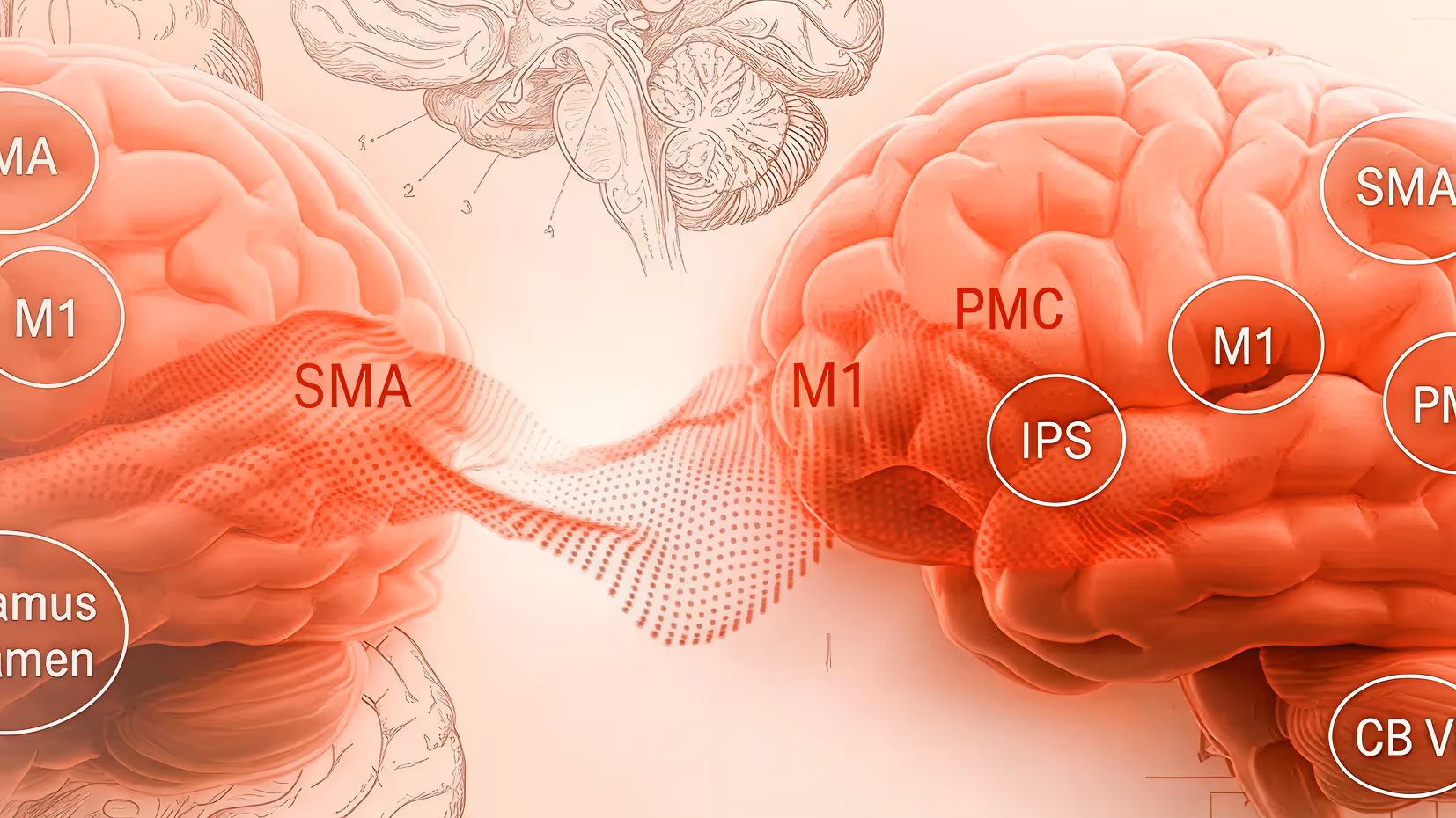
Remarkably, motor imagery activates similar brain regions and neural networks as actual movement.  The motor cortex, the area of the brain responsible for planning and executing movements, is particularly active during motor imagery. This shared neural representation suggests that imagining a movement is a powerful way to engage the brain's motor system, even without physical action.
‍

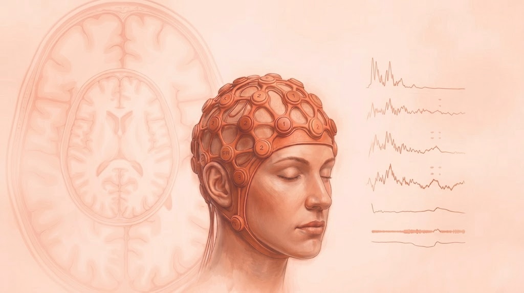
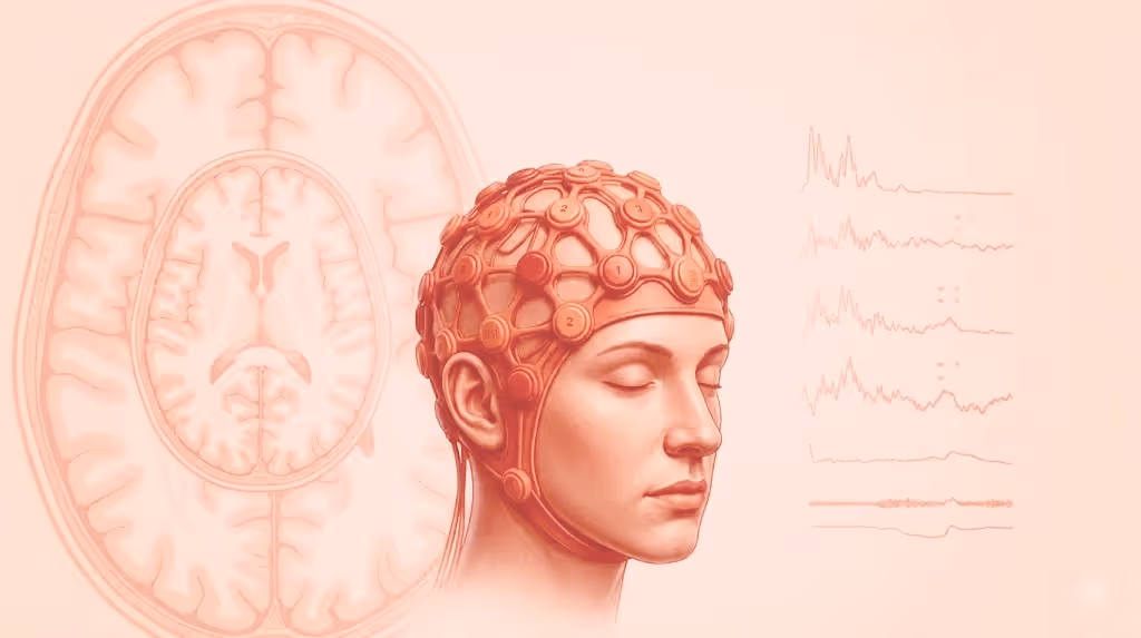
EEG Correlates of Motor Imagery: Decoding Imagined Movements
‍

Motor imagery produces characteristic changes in EEG signals, particularly over the motor cortex.  Two key features are:

‍

• Event-Related Desynchronization (ERD): A decrease in power in specific frequency bands (mu, 8-12 Hz, and beta, 13-30 Hz) over the motor cortex during motor imagery. This decrease reflects the activation of neural populations involved in planning and executing the imagined movement.
  ‍
• Event-Related Synchronization (ERS):  An increase in power in those frequency bands after the termination of motor imagery, as the brain returns to its resting state.

‍

These EEG features provide the foundation for decoding motor imagery and building BCIs that can translate imagined movements into control signals.
‍

Building a Motor Imagery BCI: A Step-by-Step Guide
‍

Now that we understand the neural basis of motor imagery, let's roll up our sleeves and build a BCI that can decode these imagined movements.  We'll follow a step-by-step process, using Python, MNE-Python, and scikit-learn to guide us.
‍

1. Loading the Dataset
‍

Choosing the Dataset: BCI Competition IV Dataset 2a

For this project, we'll use the BCI Competition IV dataset 2a, a publicly available EEG dataset specifically designed for motor imagery BCI research. This dataset offers several advantages:

‍

• Standardized Paradigm: The dataset follows a well-defined experimental protocol, making it easy to understand and replicate. Participants were instructed to imagine moving their left or right hand, providing clear labels for our classification task.
  ‍
• Multiple Subjects: It includes recordings from nine subjects, providing a decent sample size to train and evaluate our BCI model.
  ‍
• Widely Used:  This dataset has been extensively used in BCI research, allowing us to compare our results with established benchmarks and explore various analysis approaches.

‍

You can download the dataset from the BCI Competition IV website (http://www.bbci.de/competition/iv/).
‍

Loading the Data: MNE-Python to the Rescue
‍

Once you have the dataset downloaded, you can load it using MNE-Python's convenient functions.  Here's a code snippet to get you started:

‍

import mne

‍

# Set the path to the dataset directory

‍

data_path = '<path_to_dataset_directory>'

‍

# Load the raw EEG data for subject 1

‍

raw = mne.io.read_raw_gdf(data_path + '/A01T.gdf', preload=True)

‍

Replace <path_to_dataset_directory> with the actual path to the directory where you've stored the dataset files.  This code loads the data for subject "A01" from the training session ("T").
‍

2. Data Preprocessing: Preparing the Signals for Decoding
‍

Raw EEG data is often noisy and contains artifacts that can interfere with our analysis.  Preprocessing is crucial for cleaning up the data and isolating the relevant brain signals associated with motor imagery.
‍

Channel Selection: Focusing on the Motor Cortex
‍

Since motor imagery primarily activates the motor cortex, we'll select EEG channels that capture activity from this region.  Key channels include:

‍

• C3: Located over the left motor cortex, sensitive to right-hand motor imagery.
  ‍
• C4:  Located over the right motor cortex, sensitive to left-hand motor imagery.
  ‍
• Cz:  Located over the midline, often used as a reference or to capture general motor activity.

‍

# Select the desired channels

‍

channels = ['C3', 'C4', 'Cz']

‍

# Create a new raw object with only the selected channels

‍

raw_selected = raw.pick_channels(channels)
‍

Filtering:  Isolating Mu and Beta Rhythms
‍

We'll apply a band-pass filter to isolate the mu (8-12 Hz) and beta (13-30 Hz) frequency bands, as these rhythms exhibit the most prominent ERD/ERS patterns during motor imagery.

‍

# Apply a band-pass filter from 8 Hz to 30 Hz

‍

raw_filtered = raw_selected.filter(l_freq=8, h_freq=30)

‍

This filtering step removes irrelevant frequencies and enhances the signal-to-noise ratio for detecting motor imagery-related brain activity.
‍

Artifact Removal: Enhancing Data Quality (Optional)
‍

Depending on the dataset and the quality of the recordings, we might need to apply artifact removal techniques.  Independent Component Analysis (ICA) is particularly useful for identifying and removing artifacts like eye blinks, muscle activity, and heartbeats, which can contaminate our motor imagery signals.  MNE-Python provides functions for performing ICA and visualizing the components, allowing us to select and remove those associated with artifacts.  This step can significantly improve the accuracy and reliability of our motor imagery BCI.
‍

3. Epoching and Visualizing: Zooming in on Motor Imagery
‍

Now that we've preprocessed our EEG data, let's create epochs around the motor imagery cues, allowing us to focus on the brain activity specifically related to those imagined movements.
‍

Defining Epochs: Capturing the Mental Rehearsal
‍

The BCI Competition IV dataset 2a includes event markers indicating the onset of the motor imagery cues.  We'll use these markers to create epochs, typically spanning a time window from a second before the cue to several seconds after it.  This window captures the ERD and ERS patterns associated with motor imagery.

‍

# Define event IDs for left and right hand motor imagery (refer to dataset documentation)

‍

event_id = {'left_hand': 1, 'right_hand': 2}

‍

# Set the epoch time window

‍

tmin = -1  # 1 second before the cue

‍

tmax = 4   # 4 seconds after the cue

‍

# Create epochs

‍

epochs = mne.Epochs(raw_filtered, events, event_id, tmin, tmax, baseline=(-1, 0), preload=True)

‍

Baseline Correction:  Removing Pre-Imagery Bias
‍

We'll apply baseline correction to remove any pre-existing bias in the EEG signal, ensuring that our analysis focuses on the changes specifically related to motor imagery.
‍

Visualizing: Inspecting and Gaining Insights
‍

• Plotting Epochs:  Use epochs.plot() to visualize individual epochs, inspecting for artifacts and observing the general patterns of brain activity during motor imagery.
  ‍
• Topographical Maps:  Use epochs['left_hand'].average().plot_topomap() and epochs['right_hand'].average().plot_topomap() to visualize the scalp distribution of mu and beta power changes during left and right hand motor imagery. These maps can help validate our channel selection and confirm that the ERD patterns are localized over the expected motor cortex areas.
  ‍

4. Feature Extraction with Common Spatial Patterns (CSP): Maximizing Class Differences
‍

Common Spatial Patterns (CSP) is a spatial filtering technique specifically designed to extract features that best discriminate between two classes of EEG data. In our case, these classes are left-hand and right-hand motor imagery.
‍

Understanding CSP: Finding Optimal Spatial Filters
‍

CSP seeks to find spatial filters that maximize the variance of one class while minimizing the variance of the other. It achieves this by solving an eigenvalue problem based on the covariance matrices of the two classes. The resulting spatial filters project the EEG data onto a new space where the classes are more easily separable
.

Applying CSP: MNE-Python's CSP Function
‍

MNE-Python's mne.decoding.CSP() function makes it easy to extract CSP features:

‍

from mne.decoding import CSP

‍

# Create a CSP object

‍

csp = CSP(n_components=4, reg=None, log=True, norm_trace=False)

‍

# Fit the CSP to the epochs data

‍

csp.fit(epochs['left_hand'].get_data(), epochs['right_hand'].get_data())

‍

# Transform the epochs data using the CSP filters

‍

X_csp = csp.transform(epochs.get_data())
‍

Interpreting CSP Filters: Mapping Brain Activity
‍

The CSP spatial filters represent patterns of brain activity that differentiate between left and right hand motor imagery.  By visualizing these filters, we can gain insights into the underlying neural sources involved in these imagined movements.
‍

Selecting CSP Components: Balancing Performance and Complexity
‍

The n_components parameter in the CSP() function determines the number of CSP components to extract.  Choosing the optimal number of components is crucial for balancing classification performance and model complexity.  Too few components might not capture enough information, while too many can lead to overfitting. Cross-validation can help us find the optimal balance.
‍

5. Classification with a Linear SVM: Decoding Motor Imagery
‍

Choosing the Classifier: Linear SVM for Simplicity and Efficiency
‍

We'll use a linear Support Vector Machine (SVM) to classify our motor imagery data.  Linear SVMs are well-suited for this task due to their simplicity, efficiency, and ability to handle high-dimensional data.  They seek to find a hyperplane that best separates the two classes in the feature space.
‍

Training the Model: Learning from Spatial Patterns
‍

from sklearn.svm import SVC

‍

# Create a linear SVM classifier

‍

svm = SVC(kernel='linear')

‍

# Train the SVM model

‍

svm.fit(X_csp_train, y_train)
‍

Hyperparameter Tuning: Optimizing for Peak Performance
‍

SVMs have hyperparameters, like the regularization parameter C, that control the model's complexity and generalization ability.  Hyperparameter tuning, using techniques like grid search or cross-validation, helps us find the optimal values for these parameters to maximize classification accuracy.
‍

Evaluating the Motor Imagery BCI: Measuring Mind Control
‍

We've built our motor imagery BCI, but how well does it actually work? Evaluating its performance is crucial for understanding its capabilities and limitations, especially if we envision real-world applications.

Cross-Validation: Assessing Generalizability
‍

To obtain a reliable estimate of our BCI's performance, we'll employ k-fold cross-validation.  This technique helps us assess how well our model generalizes to unseen data, providing a more realistic measure of its real-world performance.

‍

from sklearn.model_selection import cross_val_score

‍

# Perform 5-fold cross-validation

‍

scores = cross_val_score(svm, X_csp, y, cv=5)

‍

# Print the average accuracy across the folds

‍

print("Average accuracy: %0.2f" % scores.mean())
‍

Performance Metrics: Beyond Simple Accuracy
‍

• Accuracy: While accuracy, the proportion of correctly classified instances, is a useful starting point, it doesn't tell the whole story.  For imbalanced datasets (where one class has significantly more samples than the other), accuracy can be misleading.
  ‍
• Kappa Coefficient: The Kappa coefficient (κ) measures the agreement between the classifier's predictions and the true labels, taking into account the possibility of chance agreement.  A Kappa value of 1 indicates perfect agreement, while 0 indicates agreement equivalent to chance. Kappa is a more robust metric than accuracy, especially for imbalanced datasets.
  ‍
• Information Transfer Rate (ITR): ITR quantifies the amount of information transmitted by the BCI per unit of time, considering both accuracy and the number of possible choices.  A higher ITR indicates a faster and more efficient communication system.
  ‍
• Sensitivity and Specificity:  These metrics provide a more nuanced view of classification performance.  Sensitivity measures the proportion of correctly classified positive instances (e.g., correctly identifying left-hand imagery), while specificity measures the proportion of correctly classified negative instances (e.g., correctly identifying right-hand imagery).
  ‍

Practical Implications: From Benchmarks to Real-World Use
‍

Evaluating a motor imagery BCI goes beyond just looking at numbers.  We need to consider the practical implications of its performance:

‍

• Minimum Accuracy Requirements:  Real-world applications often have minimum accuracy thresholds.  For example, a neuroprosthetic controlled by a motor imagery BCI might require an accuracy of over 90% to ensure safe and reliable operation.
  ‍
• User Experience:  Beyond accuracy, factors like speed, ease of use, and mental effort also contribute to the overall user experience.
  ‍

Unlocking the Potential of Motor Imagery BCIs
‍

We've successfully built a basic motor imagery BCI, witnessing the power of EEG, signal processing, and machine learning to decode movement intentions directly from brain signals. Motor imagery BCIs hold immense potential for a wide range of applications, offering new possibilities for individuals with disabilities, stroke rehabilitation, and even immersive gaming experiences.
‍

Resources for Further Reading
‍

• Review article: EEG-Based Brain-Computer Interfaces Using Motor-Imagery: Techniques and Challenges https://www.ncbi.nlm.nih.gov/pmc/articles/PMC6471241/ 
• Review article: A review of critical challenges in MI-BCI: From conventional to deep learning methods https://www.sciencedirect.com/science/article/abs/pii/S016502702200262X 
• BCI Competition IV Dataset 2a https://www.bbci.de/competition/iv/desc_2a.pdf 

From Motor Imagery to Advanced BCI Paradigms
‍

This concludes our exploration of building a motor imagery BCI. You've gained valuable insights into the neural basis of motor imagery, learned how to extract features using CSP, trained a classifier to decode movement intentions, and evaluated the performance of your BCI model.

‍

In our final blog post, we'll explore the exciting frontier of advanced BCI paradigms and future directions. We'll delve into concepts like hybrid BCIs, adaptive algorithms, ethical considerations, and the ever-expanding possibilities that lie ahead in the world of brain-computer interfaces. Stay tuned for a glimpse into the future of mind-controlled technology!

‍