BCI Kickstarter #06 : Machine Learning for BCI: Decoding Brain Signals with Intelligent Algorithms

Feature Selection: Choosing the Right Ingredients for Your BCI Model
‍

Imagine you're a chef preparing a gourmet dish. You wouldn't just throw all the ingredients into a pot without carefully selecting the ones that contribute to the desired flavor profile. Similarly, in machine learning for BCI, feature selection is the art of choosing the most relevant and informative features from our preprocessed EEG data.
‍

Why Feature Selection? Crafting the Perfect EEG Recipe
‍

Feature selection is crucial for several reasons:

‍

• Reducing Dimensionality: Raw EEG data is high-dimensional, containing recordings from multiple electrodes over time. Feature selection reduces this dimensionality, making it easier for machine learning algorithms to learn patterns and avoid getting lost in irrelevant information.  Think of this like simplifying a complex recipe to its essential elements.
  ‍
• Improving Model Performance: By focusing on the most informative features, we can improve the accuracy, speed, and generalization ability of our BCI models.  This is like using the highest quality ingredients to enhance the taste of our dish.
  ‍
• Avoiding Overfitting: Overfitting occurs when a model learns the training data too well, capturing noise and random fluctuations that don't generalize to new data. Feature selection helps prevent overfitting by focusing on the most robust and generalizable patterns.  This is like ensuring our recipe works consistently, even with slight variations in ingredients.
  ‍

Filter Methods: Sifting Through the EEG Signals
‍

Filter methods select features based on their intrinsic characteristics, independent of the chosen machine learning algorithm. Here are two common filter methods:

‍

• Variance Thresholding: Removes features with low variance, assuming they contribute little to classification.  For example, in an EEG-based motor imagery BCI, if a feature representing power in a specific frequency band shows very little variation across trials of imagining left or right hand movements, it's likely not informative for distinguishing these intentions.  We can use scikit-learn's VarianceThreshold class to eliminate these low-variance features:

‍

from sklearn.feature_selection import VarianceThreshold

‍

# Create a VarianceThreshold object with a threshold of 0.1

‍

selector = VarianceThreshold(threshold=0.1)

‍

# Select features from the EEG data matrix X

‍

X_new = selector.fit_transform(X)

‍

• SelectKBest: Selects the top k features based on statistical tests that measure their relationship with the target variable.  For instance, in a P300-based BCI, we might use an ANOVA F-value test to select features that show the most significant difference in activity between target and non-target stimuli.  Scikit-learn's SelectKBest class makes this easy:

‍

from sklearn.feature_selection import SelectKBest, f_classif

‍

# Create a SelectKBest object using the ANOVA F-value test and selecting 10 features

‍

selector = SelectKBest(f_classif, k=10)

‍

# Select features from the EEG data matrix X

‍

X_new = selector.fit_transform(X, y) 
‍

Wrapper Methods: Testing Feature Subsets
‍

Wrapper methods evaluate different subsets of features by training and evaluating a machine learning model with each subset.  This is like experimenting with different ingredient combinations to find the best flavor profile for our dish.

‍

• Recursive Feature Elimination (RFE):  Iteratively removes less important features based on the performance of the chosen estimator.  For example, in a motor imagery BCI, we might use RFE with a linear SVM classifier to identify the EEG channels and frequency bands that contribute most to distinguishing left and right hand movements.  Scikit-learn's RFE class implements this method:

‍

from sklearn.feature_selection import RFE

‍

from sklearn.svm import SVC

‍

# Create an RFE object with a linear SVM classifier and selecting 10 features

‍

selector = RFE(estimator=SVC(kernel='linear'), n_features_to_select=10)

‍

# Select features from the EEG data matrix X

‍

X_new = selector.fit_transform(X, y)
‍

Embedded Methods: Learning Features During Model Training
‍

Embedded methods incorporate feature selection as part of the model training process itself.

‍

• L1 Regularization (LASSO):  Adds a penalty term to the model's loss function that encourages sparsity, driving the weights of less important features towards zero.  For example, in a BCI for detecting mental workload, LASSO regularization during logistic regression training can help identify the EEG features that most reliably distinguish high and low workload states.  Scikit-learn's LogisticRegression class supports L1 regularization:

‍

from sklearn.linear_model import LogisticRegression

‍

# Create a Logistic Regression model with L1 regularization

‍

model = LogisticRegression(penalty='l1', solver='liblinear')

‍

# Train the model on the EEG data (X) and labels (y)

‍

model.fit(X, y)
‍

Practical Considerations: Choosing the Right Tools for the Job
‍

The choice of feature selection method depends on several factors, including the size of the dataset, the type of BCI application, the computational resources available, and the desired balance between accuracy and model complexity. It's often helpful to experiment with different methods and evaluate their performance on your specific data.
‍

Classification Algorithms: Training Your BCI Model to Decode Brain Signals
‍

Now that we've carefully selected the most informative features from our EEG data, it's time to train a classification algorithm that can learn to decode user intent, predict mental states, or control external devices. This is where the magic of machine learning truly comes to life, transforming processed brainwaves into actionable insights.
‍

Loading and Preparing Data: Setting the Stage for Learning
‍

Before we unleash our classification algorithms, let's quickly recap loading our EEG data and preparing it for training:

‍

• Loading the Dataset: For this example, we'll continue working with the MNE sample dataset. If you haven't already loaded it, refer to the previous blog for instructions.
  ‍
• Feature Extraction:  We'll assume you've already extracted relevant features from the EEG data, such as band power in specific frequency bands or time-domain features like peak amplitude and latency.
  ‍
• Splitting Data: Divide the data into training and testing sets using scikit-learn's train_test_split function:

‍

from sklearn.model_selection import train_test_split

‍

# Split the data into 80% for training and 20% for testing

‍

X_train, X_test, y_train, y_test = train_test_split(X, y, test_size=0.2, random_state=42)

‍

This ensures we have a separate set of data to evaluate the performance of our trained model on unseen examples.
‍

Linear Discriminant Analysis (LDA): Finding the Optimal Projection
‍

Linear Discriminant Analysis (LDA) is a classic linear classification method that seeks to find a projection of the data that maximizes the separation between classes. Think of it like shining a light on our EEG feature space in a way that makes the different classes (e.g., imagining left vs. right hand movements) stand out as distinctly as possible.

‍

Here's how to implement LDA with scikit-learn:

‍

from sklearn.discriminant_analysis import LinearDiscriminantAnalysis

‍

# Create an LDA object

‍

lda = LinearDiscriminantAnalysis()

‍

# Train the LDA model on the training data

‍

lda.fit(X_train, y_train)

‍

# Make predictions on the test data

‍

y_pred = lda.predict(X_test)

‍

LDA is often a good starting point for BCI classification due to its simplicity, speed, and ability to handle high-dimensional data.
‍

Support Vector Machines (SVM): Drawing Boundaries in Feature Space
‍

Support Vector Machines (SVM) are powerful classification algorithms that aim to find an optimal hyperplane that separates different classes in the feature space. Imagine drawing a line (or a higher-dimensional plane) that maximally separates data points representing, for example, different mental states.

‍

Here's how to use SVM with scikit-learn:

‍

from sklearn.svm import SVC

‍

# Create an SVM object with a linear kernel

‍

svm = SVC(kernel='linear', C=1)

‍

# Train the SVM model on the training data

‍

svm.fit(X_train, y_train)

‍

# Make predictions on the test data

‍

y_pred = svm.predict(X_test)

‍

SVMs offer flexibility through different kernels, which transform the data into higher-dimensional spaces, allowing for non-linear decision boundaries. Common kernels include:

‍

• Linear Kernel:  Suitable for linearly separable data.
  ‍
• Polynomial Kernel:  Creates polynomial decision boundaries.
  ‍
• Radial Basis Function (RBF) Kernel:  Creates smooth, non-linear decision boundaries.
  ‍

Other Classifiers: Expanding Your BCI Toolbox
‍

Many other classification algorithms can be applied to BCI data, each with its own strengths and weaknesses:

‍

• Logistic Regression: A simple yet effective linear model for binary classification.
  ‍
• Decision Trees: Tree-based models that create a series of rules to classify data.
  ‍
• Random Forests: An ensemble method that combines multiple decision trees for improved performance.
  ‍

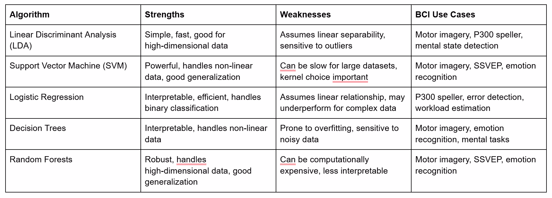
Choosing the Right Algorithm: Finding the Perfect Match
‍

The best classification algorithm for your BCI application depends on several factors, including the nature of your data, the complexity of the task, and the desired balance between accuracy, speed, and interpretability.  Here's a table comparing some common algorithms:

‍

Cross-Validation and Performance Metrics: Evaluating Your BCI Model
‍

We've trained our BCI model to decode brain signals, but how do we know if it's any good? Simply evaluating its performance on the same data it was trained on can be misleading. This is where cross-validation and performance metrics come to the rescue, providing robust tools to assess our model's true capabilities and ensure it generalizes well to unseen EEG data.
‍

Why Cross-Validation? Ensuring Your BCI Doesn't Just Memorize
‍

Imagine training a BCI model to detect fatigue based on EEG signals.  If we only evaluate its performance on the same data it was trained on, it might simply memorize the patterns in that specific dataset, achieving high accuracy but failing to generalize to new EEG recordings from different individuals or under varying conditions. This is called overfitting.

‍

Cross-validation is a technique for evaluating a machine learning model by training it on multiple subsets of the data and testing it on the remaining data. This helps us assess how well the model generalizes to unseen data, providing a more realistic estimate of its performance in real-world BCI applications.
‍

K-Fold Cross-Validation: A Robust Evaluation Strategy
‍

K-fold cross-validation is a popular cross-validation method that involves dividing the data into k equal-sized folds. The model is trained on k-1 folds and tested on the remaining fold. This process is repeated k times, with each fold serving as the test set once. The performance scores from each iteration are then averaged to obtain a robust estimate of the model's performance.

‍

Scikit-learn makes implementing k-fold cross-validation straightforward:

‍

from sklearn.model_selection import cross_val_score

‍

# Perform 5-fold cross-validation on an SVM classifier

‍

scores = cross_val_score(svm, X, y, cv=5)

‍

# Print the average accuracy across the folds

‍

print("Average accuracy: %0.2f" % scores.mean())

‍

This code performs 5-fold cross-validation using an SVM classifier and prints the average accuracy across the folds.
‍

Performance Metrics: Measuring BCI Success
‍

Evaluating a BCI model involves more than just looking at overall accuracy. Different performance metrics provide insights into specific aspects of the model's behavior, helping us understand its strengths and weaknesses.

‍

Here are some essential metrics for BCI classification:

‍

• Accuracy:  The proportion of correctly classified instances. While accuracy is a useful overall measure, it can be misleading if the classes are imbalanced (e.g., many more examples of one mental state than another).
  ‍
• Precision:  The proportion of correctly classified positive instances out of all instances classified as positive.  High precision indicates a low rate of false positives, important for BCIs where incorrect actions could have consequences (e.g., controlling a wheelchair).
  ‍
• Recall (Sensitivity):  The proportion of correctly classified positive instances out of all actual positive instances. High recall indicates a low rate of false negatives, crucial for BCIs where missing a user's intention is critical (e.g., detecting emergency signals).
  ‍
• F1-Score:  The harmonic mean of precision and recall, providing a balanced measure that considers both false positives and false negatives.
  ‍
• Confusion Matrix: A visualization that shows the counts of true positives, true negatives, false positives, and false negatives, providing a detailed overview of the model's classification performance.

‍

Scikit-learn offers functions for calculating these metrics:

‍

from sklearn.metrics import accuracy_score, precision_score, recall_score, f1_score, confusion_matrix

‍

# Calculate accuracy

‍

accuracy = accuracy_score(y_test, y_pred)

‍

# Calculate precision

‍

precision = precision_score(y_test, y_pred)

‍

# Calculate recall

‍

recall = recall_score(y_test, y_pred)

‍

# Calculate F1-score

‍

f1 = f1_score(y_test, y_pred)

‍

# Create a confusion matrix

‍

cm = confusion_matrix(y_test, y_pred) 

Hyperparameter Tuning: Fine-Tuning Your BCI for Peak Performance
‍

Most machine learning algorithms have hyperparameters, settings that control the learning process and influence the model's performance.  For example, the C parameter in an SVM controls the trade-off between maximizing the margin and minimizing classification errors.

‍

Hyperparameter tuning involves finding the optimal values for these hyperparameters to achieve the best performance on our specific dataset and BCI application. Techniques like grid search and randomized search systematically explore different hyperparameter combinations, guided by cross-validation performance, to find the settings that yield the best results.
‍

Introduction to Deep Learning for BCI: Exploring the Frontier
‍

We've explored powerful machine learning techniques for BCI, but the field is constantly evolving. Deep learning, a subfield of machine learning inspired by the structure and function of the human brain, is pushing the boundaries of BCI capabilities, enabling more sophisticated decoding of brain signals and opening up new possibilities for human-computer interaction.
‍

What is Deep Learning? Unlocking Complex Patterns with Artificial Neural Networks
‍

Deep learning algorithms, particularly artificial neural networks (ANNs), are designed to learn complex patterns and representations from data. ANNs consist of interconnected layers of artificial neurons, mimicking the interconnected structure of the brain.

‍

Through a process called training, ANNs learn to adjust the connections between neurons, enabling them to extract increasingly abstract and complex features from the data. This hierarchical feature learning allows deep learning models to capture intricate patterns in EEG data that traditional machine learning algorithms might miss.
‍

Deep Learning for BCI: Architectures for Decoding Brainwaves
‍

Several deep learning architectures have proven particularly effective for EEG analysis:

‍

• Convolutional Neural Networks (CNNs): Excel at capturing spatial patterns in data, making them suitable for analyzing multi-channel EEG recordings.  CNNs are often used for motor imagery BCIs, where they can learn to recognize patterns of brain activity associated with different imagined movements.
  ‍
• Recurrent Neural Networks (RNNs): Designed to handle sequential data, making them well-suited for analyzing the temporal dynamics of EEG signals. RNNs are used in applications like emotion recognition from EEG, where they can learn to identify patterns of brain activity that unfold over time.
  ‍

Benefits and Challenges: Weighing the Potential of Deep Learning
‍

Deep learning offers several potential benefits for BCI:

‍

• Higher Accuracy:  Deep learning models can achieve higher accuracy than traditional machine learning algorithms, particularly for complex BCI tasks.
  ‍
• Automatic Feature Learning:  Deep learning models can automatically learn relevant features from raw data, reducing the need for manual feature engineering.

‍

However, deep learning also presents challenges:

‍

• Larger Datasets: Deep learning models typically require larger datasets for training than traditional machine learning algorithms.
  ‍
• Computational Resources: Training deep learning models can be computationally demanding, requiring specialized hardware like GPUs.
  ‍

Empowering BCIs with Intelligent Algorithms
‍

From feature selection to classification algorithms and the frontier of deep learning, we've explored a powerful toolkit for decoding brain signals using machine learning. These techniques are transforming the field of BCIs, enabling the development of more accurate, reliable, and sophisticated systems that can translate brain activity into action.
‍

Resources and Further Reading
‍

• Tutorial: Scikit-learn documentation: https://scikit-learn.org/stable/
• Article: Lotte, F., Bougrain, L., Cichocki, A., Clerc, M., Congedo, M., Rakotomamonjy, A., & Yger, F. (2018). A review of classification algorithms for EEG-based brain–computer interfaces: a 10-year update. Journal of Neural Engineering, 15(3), 031005.
  ‍

Time to Build: Creating a P300 Speller with Python
‍

This concludes our exploration of essential machine learning techniques for BCI. You've gained a solid understanding of how to select relevant features, train classification models, evaluate their performance, and even glimpse the potential of deep learning.

‍

In the next post, we'll put these techniques into practice by building our own P300 speller, a classic BCI application that allows users to communicate by focusing their attention on letters on a screen. Get ready for a hands-on adventure in BCI development!

‍